A friend recently asked me a question about the delta method, which sent me briefly into a cold sweat trying to remember a concept from my first year methods sequence. In the spirit of notes to myself, here’s a post explaining what it is, why you might want to use it, and how to calculate it with R.
What is the Delta Method?
The Delta method is a result concerning the asymptotic behavior of functions over a random variable. Read asymptotics as “what happens to the thing I’m estimating as my sample gets big?”1 The usual link between random variables and a sample is that each observation in a sample that is independent and identically distributed is an observation of a random variable.
The most famous theorem I know, the Central Limit Theorem, implies that when n gets large, the distribution of the difference between the sample mean and the population mean \(\mu\) when multiplied by \(\sqrt{n}\) converges in distribution to a normal distribution \(N(0,\sigma^2)\).
Like the Central Limit Theorem, the Delta method tells us something about the asymptotic behavior of functions of random variables. Specifically, we can approximate the asymptotic behavior of functions over the random variable.
Why would I use it?
One reason as this nice post by James Pustejovsky points out is that you already do use it if you’ve ever estimated anything by 2SLS. Anytime you have a ratio estimator, the delta method is a way of construction standard errors. To be even more general, the delta method is useful in any situation where we want to form confidence intervals for nonlinear functions of parameters.
Suppose have a smooth function \(g()\) that has parameter \(\beta\) and we have an estimate \(b\) from some consistent, normally distributed estimator for the parameter, then that estimator converges to an asymptotically normal distribution. Via Taylor’s Theorem since \(g()\) is continuous and derivable up to some \(k^{th}\) derivative (\(k \geq 2\)), then at our function evaluated at \(b\) is:
\[ g(b) \approx g(\beta) + \nabla g(\beta)'(b-\beta) \]
also known as the mean value expansion. We can subtract \(g(\beta)\) from each side to get:
\[ g(b) - g(\beta) \approx \nabla g(\beta)'(b-\beta) \]
We’ll multiply both sides by \(\sqrt{n}\) because we can and because it gives us the following nice property.2 Since \(\beta\) is a constant and \(b\) is a consistent estimator for it,
\[ \sqrt{n}(g(b) -g(\beta)) \]
converges in distribution to
\[ N(0, \nabla g(\beta)^T*\sum_b * \nabla g(\beta)) \]
where the middle term represents the variance covariance matrix. That \(\nabla\) is the symbol for the gradient of the function, which is the “vector differential operator” and when applied to a function on a multi-dimensional domain is the vector of partial derivatives, which we evaluate at a given point.
The appeal of the delta method is that we get an analytic approximation of a function’s behavior by using asymptotic properties, which can be computationally pretty simple. Depending on what we’re calculated, it might actually secretly be something we’ve already been doing under a different name. Of course, we could also just bootstrap the thing, but that’s less fun now isn’t it.
I learn best by example. Show me a worked example
You bet. Consider Testa, Williams, Britzman, and Hibbing’s “Getting the Message? Choice Self-Selection, and the Efficacy of Social Movement Arguments” published in JEPS.3 The purpose of this paper is to show that designs that incorporate choice can be extended to randomize conditional on subjects’ treatment choices to answer questions of interest while preserving statistical power. Pretty cool. The authors apply the design to study how the gender of messengers for the #MeToo social movement conditions 1) who receives the message and 2) how they respond. The Estimand of interest in one part of their design is an Average Choice-Specific Treatment Effect (ACTE), which is found by taking a weighted average of an outcome in the selection condition and the average of those in the experimental control, and then dividing this estimate by the proportion of people seeking treatment.
What does that mean for the delta method? Well it means that the authors have a ratio estimate!
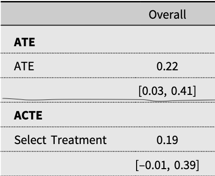
The authors find that in their design the estimate of the ACTE for the full sample on specific support for the #MeToo movement is 0.19 with a confidence interval of [-0.01, 0.39].
How did they get those numbers? Trust me when I tell you that this is an interesting paper and you should read it. The extremely short version is that they estimate a function \(g(x,y) = \frac{x}{y}\). To get a confidence interval via the delta method, we need to find the standard deviation of the asymptotic distribution of this estimator, which is equivalent to the square root of the variance of the distribution. From above, we know that we need get three terms \(\nabla g(\beta)\), the variance covariance matrix, and \(\nabla g(\beta)'\).
Let’s go in order. The gradient is just the vector of all the partial derivatives of \(g(x,y)\) with respect to each variable.
\[ \nabla g(\beta) =\begin{bmatrix} \frac{1}{y} \\ \frac{-x}{y^2} \end{bmatrix} \]
Plugging in the authors’ estimates of x and y and evaluate each of the partial derivatives at our estimates we have:
\[ \nabla g(b) =\begin{bmatrix} \frac{1}{.813} \approx 1.23 \\ \frac{-.1532}{.813^2} \approx -0.23 \end{bmatrix} \]
The variance covariance matrix here is just the variances of x and y on the diagonals because due to the randomization the covariance terms are 0. Once again plugging in the authors’ estimates of these terms:
\[ \sum_b =\begin{bmatrix} \sigma_x^2 \approx .07 & 0 \\\\ 0 & \sigma_y^2 \approx -0.0002 \end{bmatrix} \]
Great, now we have all three terms (since one is just the transpose of something we know). Now we do some matrix multiplication.
\[ \begin{align} V[b] &= \nabla g(b)^T\sum_b \nabla g(b) \\\\ V[b] &= .010 \\\\ SE[b] &= \sqrt(V[b]) \\\\ SE[b] &= .102 \end{align} \]
Being lazy and using the rule of thumb that a 95% CI critical value is 1.96:
\[ \begin{aligned} \theta &\pm 1.96*.102 \\\\ \theta &\pm \approx .2 \\\\ .19 &\pm \approx .2 \end{aligned} \]
which works out to the the confidence interval in the paper.
I have to do this in R. Show me a worked example
There’s actually a lot going on to get the weighted average estimates, but I’ll put that aside for a separate post about weighted variances. For now, note that we can note that a general property is that the gradient is a special case of the Jacobian when the function is a scalar.4 The function that I know of to calculate numerical derivatives in R is numDeriv::jacobian. This function requires us to pass a function argument, so I first make a function called ratio for this purpose.
## function that we seek to estimate
## pass this to the jacobian function
## which calculates the gradient
ratio <- function(x){
  x[1]/x[2]
}


## this function by default will output this in
## transpose form, so take the transpose to match
## discussion above
grad_g <- t(numDeriv::jacobian(func = ratio,
                               c(.153, .853)))

## Variance covariance matrix
vcov <- diag(c(0.07,0.0002)^2)

## Estimate the standard error
se_b <- sqrt(t(grad_g) %*% vcov %*%grad_g)
Now all that is left to do is calculate the confidence interval:5
estimate = .19
lwr_b = estimate - 1.96*se_b
upp_b = estimate + 1.96*se_b| x | |
|---|---|
| estimate | 0.19 |
| lwr_b | -0.01 |
| upp_b | 0.39 |
Voila. Confidence Intervals.
With extreme apologies to Wooldridge (2010).↩︎
Cameron and Trevedi (2005, p. 231); Wooldridge (2010, p. 45)↩︎
https://paultesta.org/publication/testa-2020-a/testa-2020-a.pdf↩︎
Thanks Stack Exchange.↩︎
Replication note. The actual calculations in the paper are far more precise. Running this code exactly will give you different confidence intervals due to this fact. This is not a problem for the original paper, but rather is due to purposefully simplifying on my end.↩︎