Building Up from our Bootstraps

Thinking about Learning Methods

Note to Readers: If you arrived at this post because of a search query about how to do bootstrapping, especially wild bootstrapping, in R, skip to the Replication example section at the bottom.

When I first entered grad school, I knew little to nothing about quantitative methods. The methods sequence at Berkeley was daunting to me, and I felt overwhelmed with all of the new skills and techniques that my cohort seemed to be picking up with ease.¹

What was intimidating? In general, a slide that looked like this:

Over time, these slides became less scary to me, and I *think* I know why. As I got a bit better at methods, I started translating them into implementations in code. Very often, the code implementation made more sense to me. Admittedly, such a learning style has downsides. Methods are a language, and language learners are correctly deterred from trying to translate too much between languages. However, I knew very little. When starting out, I *needed* to make those connections so that eventually, I could read and understand those slides without having to resort to a multi-step process. In short, I needed a bootstrap.

In this post, I am going to give a walk-through of the method by explaining how to well, bootstrap. Introduced by Efron (1979)², the bootstrap is a method for estimating the distribution of a test statistic via repeated resampling of data or a model estimated from data.³ Unreasonably effective in multiple applications, the bootstrap provides approximations to the distribution of test statistics, confidence intervals, and rejection probabilities. Extended by other authors, the procedure also works for the situation where the original assumption of independent and identically distributed errors does not hold.

Why would you be interested in knowing any of these points? Simply put, we do not believe that the data we have from any given experiment or study is complete. Furthermore, we know that when we run the experiment or study again, we are liable to get different data each time. In order to infer a relationship from data, we have to do something about this fundamental uncertainty. Efron’s initial insight was that there are times when we can use the data we have as a population and simulate replications. Since we already have a guess about the mechanism that creates the data (our model!), why not trust it and use it to generate data that we hypothesize should have the same distribution as the real data. Do that many times, and we get a sampling distribution. From that sampling distribution, we can draw inferences and insights.

Except if you are me learning about this originally, that was not so clear. Here is what I did when I was trying to learn what was going on.

Code

Strangely enough, I started with code. Partially this is because I knew a little bit more code than I did math.⁴ The other reason is that seeing how the code was written provided intuition as to what the math meant.⁵ Here’s the general process for bootstrapping.

1. Get some data

2. Get the answer to something you care about. Take that as the statistic of interest. This might be an average, a standard error, or something more complicated with more Greek letters.

3. Use the model to generate a bunch of new samples by sampling the data you have repeatedly with replacement.

4. For each one of those samples, compute the same thing you cared about in (2). This is the *sampling distribution* of the bootstrap.

5. Use the results from (3) and (4) to (usually) take an average or a standard deviation of that sample distribution. That is your bootstrapped estimate.

The textbook case⁶ is bootstrapping the sample mean.

set.seed(12)
## Get some data 
N <- 100
data <- rnorm(N, mean = 10, sd = 2)

## Get a statistic 
sample_mean <- mean(data)
sample_mean 

## [1] 9.937663

## Number of Bootstrap replications 
B <- 10000
bootstrap_means <- vector(mode = "logical", 
                          length = B)
## repeatedly sample the data with replacement 
## for each repetition take the sample mean 
for(i in 1:B){
    bootstrap_means[i] <- mean(sample(data, 
                                      size = N, 
                                      replace = TRUE))
}


## Take the average and standard deviations 
sample_mean_bootstrap <- mean(bootstrap_means)
sample_se_bootstrap <- sd(bootstrap_means)

sample_mean_bootstrap

## [1] 9.935817

sample_se_bootstrap

## [1] 0.1710695

ggplot(data = tibble(
    bootstrap_means = bootstrap_means), 
       aes(x = bootstrap_means))+
    geom_histogram()+
    geom_vline(xintercept = mean(bootstrap_means))+
    theme_minimal()+
    xlab("Replicates")+
    ylab("Count")+
    ggtitle("Bootstrap Distribution")

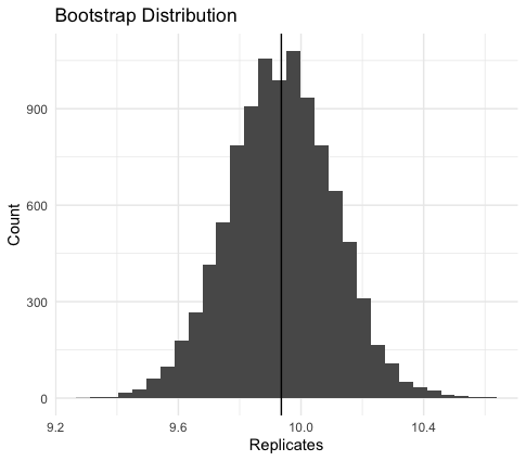
Note that in this case, the original sample mean and the bootstrapped sample mean are functionally identical. If I had run more replicates, the procedure for the sample mean is unbiased so would be identical in convergence. The bootstrap standard error gives the uncertainty of this estimate for the data.

Why did I think this kind of exercise worked for me? Well, in part, it is because I already knew the answer, so all I had to do was fill in the appropriate steps. It turns out that this idea actually has some support in theories of learning and some success in classrooms. In my undergraduate class on Applied Causal Inference, I experimented with it on the final two assignments and saw great improvement from students. My pet theory is that knowing where one needs to go is empowering for learning. Additionally, it becomes easier to take the next steps to determine why something is correct once you know that your solution is correct. That allowed me to turn towards the intuition of the problem.

Intuition

Let’s go back to the results we found. We have an answer to the question of an estimate of the standard error of the sample mean, but there are some open questions from that simulation. For one, why do we draw from the same data with replacement? And why is it that we take a sample exactly the same size? For that matter, is this distribution actually what we want? Our sample isn’t all the data on our variable of interest. That’s why it is a sample!

The intuition for the first question is that in the simulation, we imagine all of the different ways we could have drawn 50 observations from a set of numbers. We are, in effect, making many new populations. If we did not set replacement equal to true, we’d get the same sample every time, just in different orders. However, that same point implies a restriction on this bootstrap procedure. We have to have a reason to believe that the thing we want to know comes from a sample where the draws of data are independent and identically distributed. If we set replace to FALSE, the data draws would not be independent. They have to be identically distributed because they are assumed to come from our original sample.

The short answer to the third question is no. What we actually want is many draws from the real data generating process. We do not have that. If we did have that, we would not go through any of this trouble to write out a bunch of formulas. We would just say, “It’s 7” and move on with our lives.⁷ What we have is the empirical distribution associated with our original sample of data.⁸

At this point in a textbook or a lecture, the professor usually makes a point that the bootstrap is not perfect and can fail. Our graph of the empirical distribution looks normally distributed, which crops up whenever the underlying process follows the Weak Law of Large Numbers and the Central Limit Theorem. That suggests that our code is tapping into a process that requires our estimator (here, the sample mean) to be approximately linear and normal. If what we were dealing with was not both, then we are not simulating the right process.

Except at this point, we should worry a little bit if we bootstrap something more complicated than a sample mean. A difficulty with a lot of homework assignments and methods learning is what I refer to as the “draw the owl” problem.

Most problems we see are not as simple as getting the standard error of a sample mean when we claim independent and identically distributed errors. For many important problems, and frankly basically everything in everyday life, the errors are correlated in some way. Most problems political scientists study have correlated error structures. Voting reform efforts in one state in the United States may or may not affect voters in a different state. Nonetheless, every voter in the state with a voting reform is “treated” to that reform. If you have 4,000,000 voters in a state, the number of effective observations you have is still one state. Beyond that, political scientists love regression models and, to be more specific, models estimated via ordinary least squares. So do the economists. Does the bootstrap not apply in the cases?

Getting Wild with the Bootstrap

Surprisingly with a slight modification, we can use the bootstrap when we have a non-constant variance of the error terms (or if one is feeling fancy heteroskedastic errors). The term of art for these bootstrap models is the “wild” bootstrap.⁹

What do we do in a wild bootstrap? We have some linear model

$$ Y_i = \hat{\beta}\textbf{X}_i + \epsilon_i $$

where the error term has a variance that is unknown and (potentially) heteroskedastic. The wild bootstrap does the same thing as the regular bootstrap in terms of steps. The difference is how we generate the new data. Instead of generating new data each time in the previous way, we instead hold the covariates fixed from the original data and generate new errors for our bootstrap replicates by first multiplying the residuals by a random variable and then generating new residuals. The covariates are not resampled. We then randomly select new residuals for each data point. This will result in a new outcome value for each observation.

From this point, we generate a bootstrap sample, estimate the linear model using this sample, compute the statistic of interest, obtain the empirical distribution by repeating the process many times, and then use that distribution for our tests.

For reasons that are described in more detail in texts, the new random variable tends to come from a Rademacher distribution.¹⁰

From a learning perspective, the reason I eventually understood what was going on with the wild bootstrap, and my understanding is still pretty limited, was that I built upon what I had previously known. Karl Polya’s brilliant text How to Solve It mentions that as a problem-solving strategy, a good first step is to simply ask, “Have I seen this before? If I have, is anything different than when I saw it before?”

In many ways, this is no different than my baseball practice when I was little. Start by learning to swing a baseball bat without a ball. Add the ball, but just on a tee. Move the ball from being on the tee to being underhand lobbed by a coach. Move the ball from lobs to slow pitches from ~20 feet away. Move the ball to slow pitches from the mound. Move the ball to regular speed pitches from the mound. Whenever an issue was found, diagnose by running through similar steps, starting with an easier version of the problem.

My learning built on the foundation of being comfortable with an easier problem that I had solved, and then I saw the same type of problem with a new twist. Most of the progress I made came from this type of deliberate practice and from problems that I found that were explicit about slowing adding new steps. As Allen Iverson would say:

Practice is not the game. Methods learning is not about immediately applying to research (though that does help), but problems have to ramp up in an intelligent manner. After designing and teaching a methods course for the first time, I found writing good problems to be the hardest and most time-consuming part of course prep.

Replication Example

I am going to use the data from Adam Scharpf and Christian Gläßel’s article in the American Journal of Political Science Why Underachievers Dominate Secret Police Organizations: Evidence from Autocratic Argentina, which I happen to like a great deal. The paper is interested in who serves in secret police forces, and the authors argue that security officials with weak early career performances join secret police to signal their value to regime leaders. Using data from Argentina, they test the effect of Graduation rank on whether an individual served in Battalion 601, which was the most powerful secret police organization. The paper uses logistic regression, but I am going to work with a plain old linear probability model. I refer to their dataset as police, and the data looks like the following.

bn601	gradrank	cavalry	infantry	avglit	academage	cohort
0	3.404255	0	0	0.7628371	214	77
0	4.680851	1	0	0.9685043	230	77
0	5.531915	0	0	0.9698494	212	77
0	5.957447	0	0	0.7044107	216	77
0	6.382979	0	1	0.7628371	215	77
0	7.659574	0	0	0.9685043	239	77

I will replicate Model 3 in Table 1 of the AJPS paper using the amazing fixest lmtest and sandwich packages. fixest is as the kids would say “stupid good” and blazingly fast. The other two packages are to perform standard error adjustments on the fly.

This model includes variables for whether an officer was a cavalry officer, an infantry officer, the home literacy rate, and cadet age. The standard errors are heteroskedastic and clustered by cohorts. The first model is a replication of the model in the paper. The second is the equivalent OLS model. I will show bootstrapped errors on the latter.

origModel <- feglm(bn601 ~ gradrank + 
                       cavalry + 
                       infantry+
                       avglit + 
                       academage, 
                   data = police, cluster = ~cohort, 
                   family = "logit")
lpmVersion <- feols(bn601 ~ gradrank + cavalry + 
                        infantry+
                        avglit + academage, 
                    data = police, cluster = ~cohort)

Table 1: Replication of Model 3 from Scharpf and Gläßel

	Original	LPM
(Intercept)	−5.51345***	−0.03580
	(1.53594)	(0.04841)
gradrank	0.01360***	0.00045**
	(0.00380)	(0.00016)
cavalry	−0.55128+	−0.01347*
	(0.30813)	(0.00641)
infantry	0.51680**	0.01958*
	(0.17105)	(0.00724)
avglit	1.29053+	0.04371+
	(0.69447)	(0.02303)
academage	0.00108	0.00004
	(0.00600)	(0.00019)
Num.Obs.	4216	4216
R2		0.010
R2 Adj.		0.008
R2 Within
R2 Pseudo	0.032
AIC	1272.7	−2254.7
BIC	1310.8	−2216.6
Log.Lik.	−630.364	1133.346
Std.Errors	by: cohort	by: cohort
+ p < 0.1, * p < 0.05, ** p < 0.01, *** p < 0.001

As can be seen, we can nearly perfectly replicate the model in the paper and the LPM gives the same general answer regarding significance, which is less important here.

Let’s now run several different standard errors, using a trick that I got from Grant McDermott. The first type is the type reported in the paper, heteroskedastic errors clustered by cohort. The second and third are two different wild bootstraps using the Rademacher and Mammen distributions to draw the variable to modify the residuals.

lpmV <- lm(bn601 ~ gradrank + cavalry + 
                        infantry+
                        avglit + academage, 
                    data = police)
vcovs <- list(
"Heteroskedastic Clustered" = vcovCL(lpmV, 
                                     cluster = ~ cohort),

"BS-wild-cluster" = vcovBS(lpmV, 
                           cluster = ~cohort, 
                           R = 500, 
                           type = "wild-rademacher"),

"BS-wild-cluster-mammen" = vcovBS(lpmV, 
                                  cluster = ~cohort, 
                                  R = 500, 
                                  type = "mammen")
)

models <- lapply(vcovs,function(x) coeftest(lpmV, vcov =x))

Table 2: Scharpf and Gläßel LPM Models with different standard errors

	Heteroskedastic Clustered	BS-wild-cluster	BS-wild-cluster-mammen
(Intercept)	−0.03580	−0.03580	−0.03580
	(0.04841)	(0.04747)	(0.04732)
gradrank	0.00045**	0.00045**	0.00045**
	(0.00016)	(0.00016)	(0.00016)
cavalry	−0.01347*	−0.01347*	−0.01347*
	(0.00641)	(0.00680)	(0.00660)
infantry	0.01958**	0.01958**	0.01958**
	(0.00724)	(0.00729)	(0.00705)
avglit	0.04371+	0.04371+	0.04371+
	(0.02303)	(0.02303)	(0.02253)
academage	0.00004	0.00004	0.00004
	(0.00019)	(0.00018)	(0.00019)
Num.Obs.	4216	4216	4216
AIC	−2252.7	−2252.7	−2252.7
BIC	−2208.3	−2208.3	−2208.3
Log.Lik.	1133.346	1133.346	1133.346
+ p < 0.1, * p < 0.05, ** p < 0.01, *** p < 0.001

If you’re using Stata, or have a co-author who feels the urge to use R packages that are ports from Stata packages, then boottest is the package that you want. The Stata Journal article is here.

Conclusion

Methods can be hard, and often make me feel like I know very little about the world. Today, I tend to like that feeling because I have developed a tool or two over time to push forward in my own learning. For those who feel lost now, do not despair. I was where you are now, and frequently still am. What I would strongly encourage is to find your own bootstrapping process for learning.