Introduction
This simulation is an example of randomization inference.
set.seed(8675309)
library(dplyr)
library(ggplot2)
library(readr)
To understand how the public perceives Donald Trump’s tweets, YouGov runs a poll that asks a representative sample of the US population to rate each tweet the day they are published. Trump’s writing style when tweeting is often hyperbolic, with certain words in all-caps and extending out others (“sooooo”) for effect.
To show how randomization inference works, let’s simulate some Trump tweets based on the YouGov scoring system. Further, let’s suppose for the sake of argument that Trump randomly inserts hyperbolic phrases into his tweets.
# Generate some tweets
tweets <- data.frame(tweet = c(1:20),
                     score_obs = round(rnorm(20, 0, 36)),
                     exclamation = sample(0:1, 20, replace = T))%>%
    mutate(Y_i1 = ifelse(exclamation == 1, score_obs, NA),
           Y_i0 = ifelse(exclamation == 0, score_obs, NA))
glimpse(tweets)
## Observations: 20
## Variables: 5
## $ tweet       <int> 1, 2, 3, 4, 5, 6, 7, 8, 9, 10, 11, 12, 13, 14, 15, 1…
## $ score_obs   <dbl> -36, 26, -22, 73, 38, 36, 1, 24, 21, 33, -56, 37, 5,…
## $ exclamation <int> 0, 0, 0, 1, 1, 0, 1, 1, 1, 0, 1, 0, 1, 1, 1, 0, 0, 1…
## $ Y_i1        <dbl> NA, NA, NA, 73, 38, NA, 1, 24, 21, NA, -56, NA, 5, -…
## $ Y_i0        <dbl> -36, 26, -22, NA, NA, 36, NA, NA, NA, 33, NA, 37, NA…
For this simulation, exclamation is a treatment assignment and we want to know the effect that it has on the score of the tweets.
Sharp Null Hypothesis
# Fill in potential outcomes to make the Sharp Null
tweets_ri = tweets %>%
    mutate(Y_i1 = ifelse(is.na(Y_i1), Y_i0, Y_i1),
           Y_i0 = ifelse(is.na(Y_i0), Y_i1, Y_i0))%>%
    select(Y_i1, Y_i0, exclamation, score_obs)
glimpse(tweets_ri)
## Observations: 20
## Variables: 4
## $ Y_i1        <dbl> -36, 26, -22, 73, 38, 36, 1, 24, 21, 33, -56, 37, 5,…
## $ Y_i0        <dbl> -36, 26, -22, 73, 38, 36, 1, 24, 21, 33, -56, 37, 5,…
## $ exclamation <int> 0, 0, 0, 1, 1, 0, 1, 1, 1, 0, 1, 0, 1, 1, 1, 0, 0, 1…
## $ score_obs   <dbl> -36, 26, -22, 73, 38, 36, 1, 24, 21, 33, -56, 37, 5,…
First we take a difference in means in our observed values, our average treatment effect (ATE). We are going to compare this value to a distribution created by randomizing treatment assignment under the assumption that the true potential outcomes are identical and so there is no difference in treatment and control. This is the Sharp Null Hypothesis.
ATE = mean(tweets_ri$score_obs[tweets_ri$exclamation == 1]) - mean(tweets_ri$score_obs[tweets_ri$exclamation == 0])
ATE
## [1] -8
Simulation
To apply randomization inference, we first create all possible treatment vectors.
poss_treatments = matrix(NA, 10000, 20)
for(i in 1:nrow(poss_treatments)){
    poss_treatments[i,] = sample(tweets_ri$exclamation, 20, replace = F)
}

# Keep only unique treamtent assignments
poss_treatments = unique(poss_treatments)
Next we calculate the average treatment effect for each possible randomization
poss_ate = NA
for(i in 1:nrow(poss_treatments)){
    mean_w_exclam = mean(tweets_ri$score_obs[poss_treatments[i,]== 1])

    mean_wo_exclam = mean(tweets_ri$score_obs[poss_treatments[i, ]== 0])

    poss_ate[i] = mean_w_exclam - mean_wo_exclam
}
To evaluate whether our observed average treatment effect is significant, we can plot the distribution of our randomization. Code for that is given below.
Results
ggplot(as.data.frame(poss_ate), aes(x = poss_ate))+
    geom_histogram(aes(y=..density..), binwidth = 1)+
    geom_vline(xintercept = ATE, color = "red", size = 1)+
    theme_minimal()+
        xlab("Randomized Average Treatment Effects")+
        ylab("Density")+
        ggtitle("Randomization Inference of the Effect of Exclamations\nin Donald Trump's Tweets")
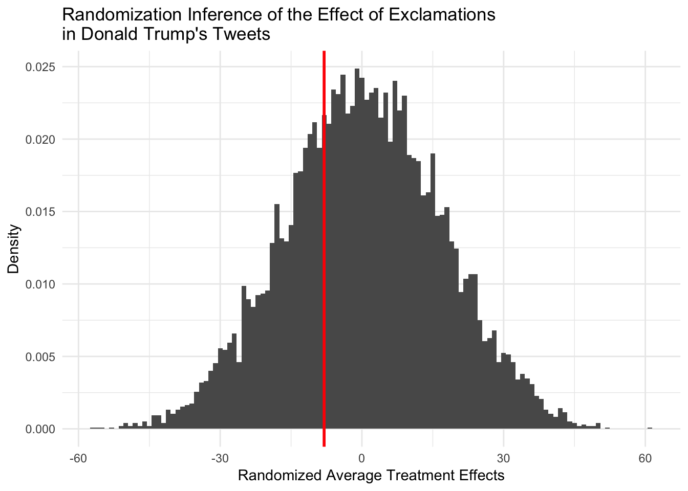
Now, we can also calculate a p-value.
# One tailed
sum(poss_ate>=ATE)/length(poss_ate)
## [1] 0.6925842
or a Two tailed p-value.
# Two tailed
sum(abs(poss_ate)>=ATE)/length(poss_ate)
## [1] 1
Given how we created our data, it is unsurprising that the p-value is not signficant. What is practically helpful is the procedure for simulation.